Importing and visualising EEG data
Below we import and reshape EEG data from the eegkit package.
library(neurogam)
library(ggplot2)
library(eegkit)
library(dplyr)

# retrieving some EEG data
data(eegdata)
head(eegdata)
#>       subject group condition trial channel time voltage
#> 1 co2a0000364     a        S1     0     FP1    0  -8.921
#> 2 co2a0000364     a        S1     0     FP1    1  -8.433
#> 3 co2a0000364     a        S1     0     FP1    2  -2.574
#> 4 co2a0000364     a        S1     0     FP1    3   5.239
#> 5 co2a0000364     a        S1     0     FP1    4  11.587
#> 6 co2a0000364     a        S1     0     FP1    5  14.028

# plotting the average ERP per group and channel
eegdata |>
    summarise(voltage = mean(voltage), .by = c(group, channel, time) ) |>
    ggplot(aes(x = time, y = voltage, colour = group) ) +
    geom_line() +
    facet_wrap(~channel) +
    theme_bw()
# retrieving sensors x and y coordinates
data(eegcoord)
enames <- rownames(eegcoord)

# merging the data
eeg_coords <- eegcoord |>
    mutate(channel = enames) |>
    select(channel, xproj, yproj)

# summarising the data
eeg_data <- eegdata |>
    summarise(voltage = mean(voltage), .by = c(subject, channel, time) ) |>
    left_join(eeg_coords, by = "channel") |>
    # converting timesteps to seconds
    mutate(time = (time + 1) / 256) |>
    # rounding numeric variables
    mutate(across(is.numeric, ~round(.x, 4) ) ) |>
    # removing NAs
    na.omit() |>
    # scaling the variables before fitting
    mutate(
        xproj = xproj / sd(xproj),
        yproj = yproj / sd(yproj),
        voltage = voltage / sd(voltage)
        )

# sensors: one row per channel with columns xproj, yproj
sensors <- unique(eeg_data[, c("channel", "xproj", "yproj")])

# show a few rows
head(sensors)
#>      channel      xproj     yproj
#> 1        FP1 -0.6712590 1.8012175
#> 257      FP2  0.6721339 1.7996850
#> 513       F7 -1.4744817 0.9956874
#> 769       F8  1.4718131 0.9941358
#> 1025     AF1 -0.3442040 1.4196194
#> 1281     AF2  0.3450789 1.4182019
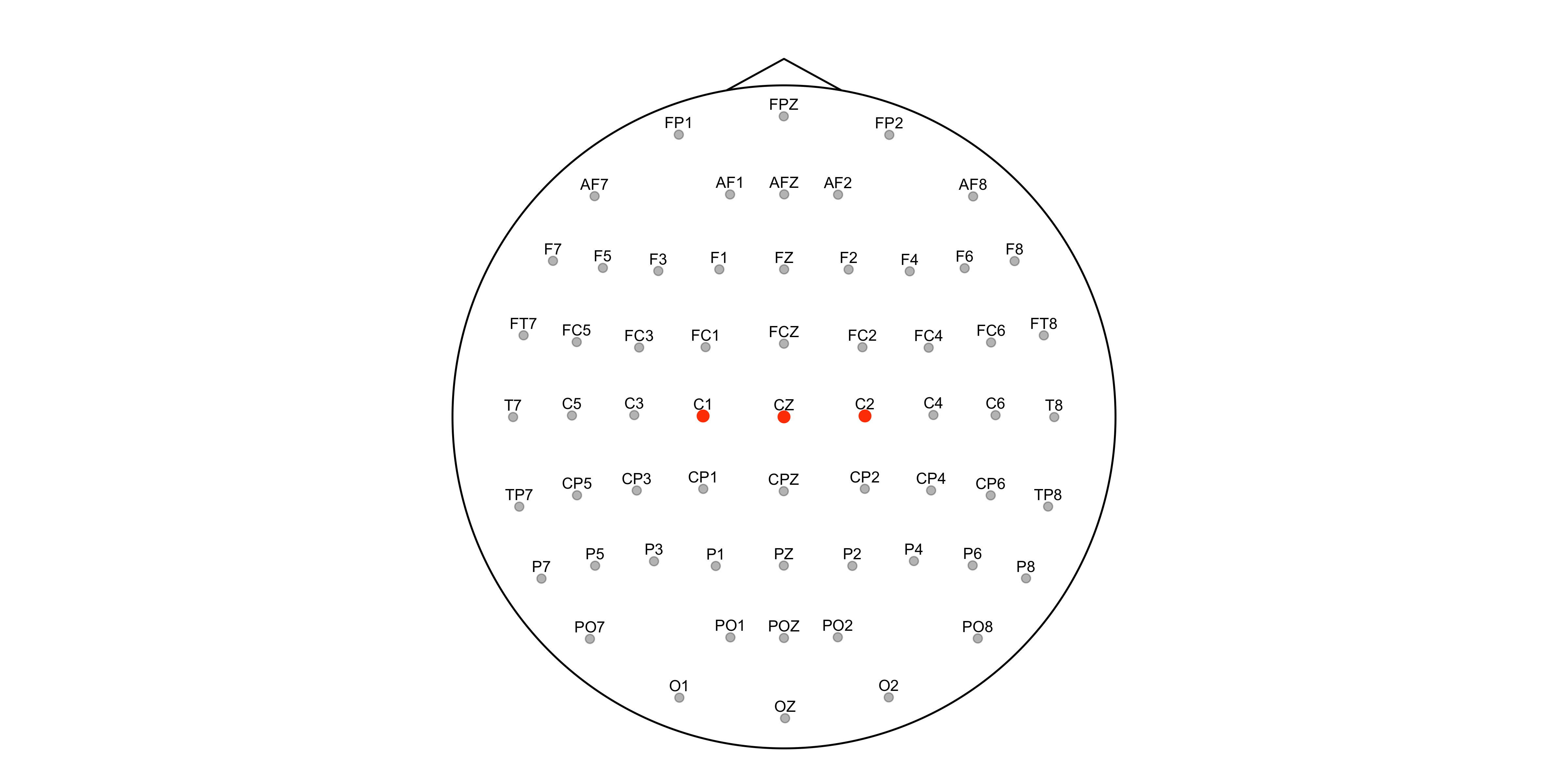
We visualise the sensors grid using the plot_sensors() function.
# plotting the sensors grid
plot_sensors(
    sensors,
    show_points = TRUE,
    show_labels = TRUE,
    label_col = "channel",
    label_repel = FALSE,
    highlight = c("C1", "CZ", "C2"),
    label_only_highlight = FALSE,
    dim_others = TRUE,
    head_expand = 1.1
    )
We visualise the average EEG topography through time using the plot_eeg() function.
# retrieving the first 100 unique timesteps
time_steps <- unique(eeg_data$time)[1:100]

# taking 8 equally spaced timesteps
time_steps_discrete <- st_take_n_times(time_vec = time_steps, N = 8)

# averaging EEG data per channel and timestep
eeg_data_summary <- eeg_data %>%
    summarise(voltage = mean(voltage), .by = c(channel, time, xproj, yproj) ) |>
    dplyr::filter(time %in% time_steps_discrete)

# topoplot of summary data
plot_eeg(
    x = eeg_data_summary,
    type = "topo",
    sensors = sensors,
    times = time_steps_discrete,
    grid_res = 200,
    value_col = "voltage",
    facet_nrow = 2,
    # fill_limits = c(-2, 2)
    fill_limits = "global_quantile"
    )
Spatio-temporal modelling with BGAMs
In progress.