Importing and visualising EEG data
Below we import and reshape EEG data from the eegkit package.
library(patchwork)
library(neurogam)
library(ggplot2)
library(eegkit)
library(dplyr)
# retrieving some EEG data
data(eegdata)
head(eegdata)
#> subject group condition trial channel time voltage
#> 1 co2a0000364 a S1 0 FP1 0 -8.921
#> 2 co2a0000364 a S1 0 FP1 1 -8.433
#> 3 co2a0000364 a S1 0 FP1 2 -2.574
#> 4 co2a0000364 a S1 0 FP1 3 5.239
#> 5 co2a0000364 a S1 0 FP1 4 11.587
#> 6 co2a0000364 a S1 0 FP1 5 14.028
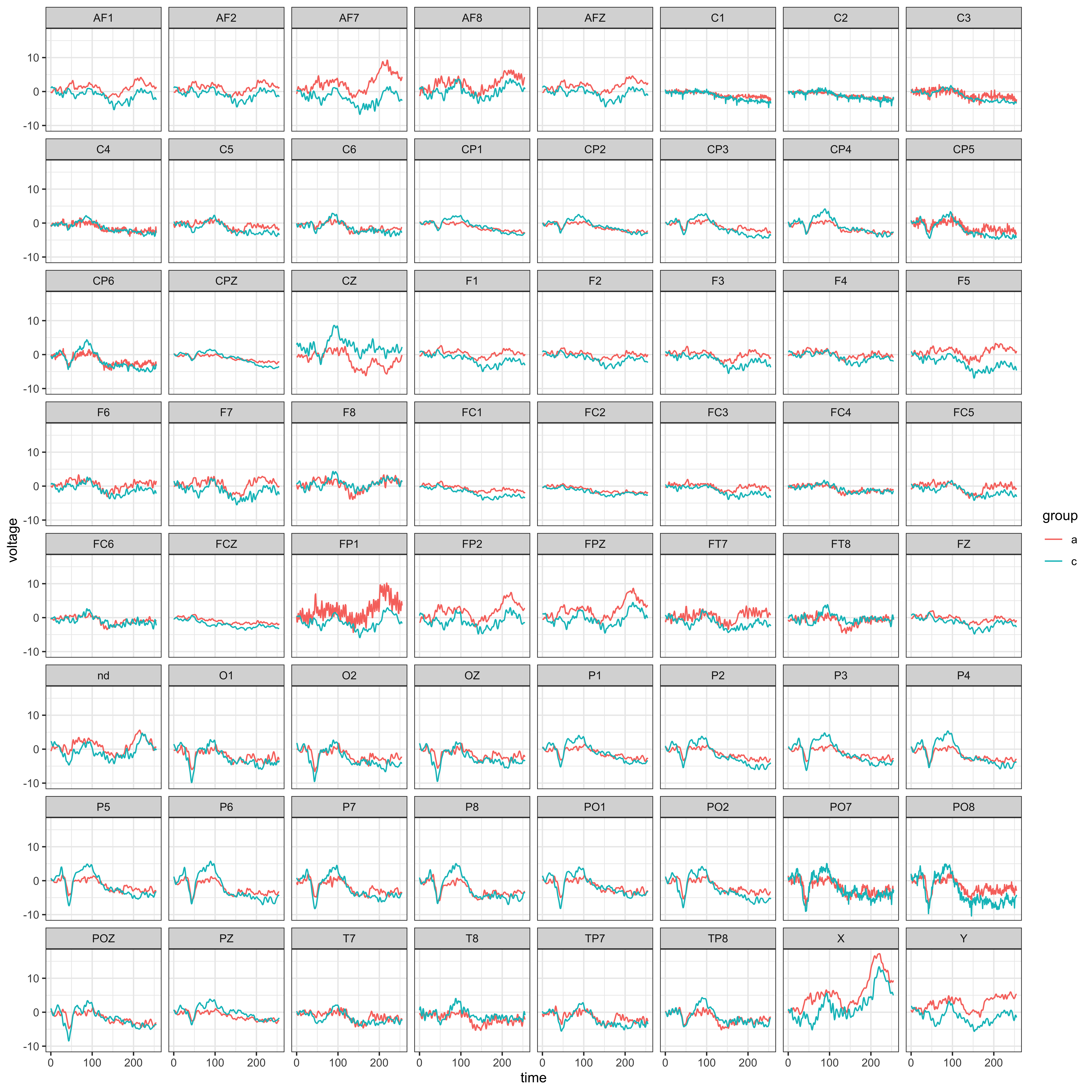
# plotting the average ERP per group and channel
eegdata |>
summarise(voltage = mean(voltage), .by = c(group, channel, time) ) |>
ggplot(aes(x = time, y = voltage, colour = group) ) +
geom_line() +
facet_wrap(~channel) +
theme_bw()
# reshape the data
eeg_data <- eegdata |>
    # keeping only one channel
    dplyr::filter(channel == "PZ") |>
    # converting timesteps to seconds
    mutate(time = (time + 1) / 256) |>
    # rounding numeric variables
    mutate(across(where(is.numeric), ~ round(.x, 4) ) ) |>
    # removing NAs
    na.omit()

# show a few rows
head(eeg_data)
#>       subject group condition trial channel   time voltage
#> 1 co2a0000364     a        S1     0      PZ 0.0039  -2.797
#> 2 co2a0000364     a        S1     0      PZ 0.0078  -4.262
#> 3 co2a0000364     a        S1     0      PZ 0.0117  -4.262
#> 4 co2a0000364     a        S1     0      PZ 0.0156  -2.797
#> 5 co2a0000364     a        S1     0      PZ 0.0195  -0.844
#> 6 co2a0000364     a        S1     0      PZ 0.0234   0.132
Fitting a first model
We fit the model (a BGAMM) on one channel (PZ) to test for group difference at every timestep.
# fitting the BGAMM to identify clusters
results1 <- testing_through_time(
    # EEG data
    data = eeg_data,
    # participant column
    participant_id = "subject",
    # EEG column
    outcome_id = "voltage",
    # no predictor
    predictor_id = NA,
    # basis dimension
    kvalue = 20,
    # we recommend fitting the GAMM on summary statistics (mean and SD)
    multilevel = "summary",
    # no by-participant varying smooth (for speed purposes)
    varying_smooth = FALSE,
    # threshold on posterior odds
    threshold = 10,
    # number of MCMCs
    chains = 4,
    # number of parallel cores
    cores = 4,
    # number of warmup iterations
    warmup = 1000,
    # total number of iterations (per chain)
    iter = 2000
    )
Visualising the results
# displaying the identified clusters
print(results1)
#>
#> ==== Time-resolved GAM results ================================
#>
#> Clusters found: 4
#>
#>      sign id onset offset duration
#>  positive  1 0.004  0.016    0.012
#>  positive  2 0.316  0.430    0.114
#>  negative  1 0.144  0.215    0.071
#>  negative  2 0.727  1.000    0.273
#>
#> =================================================================
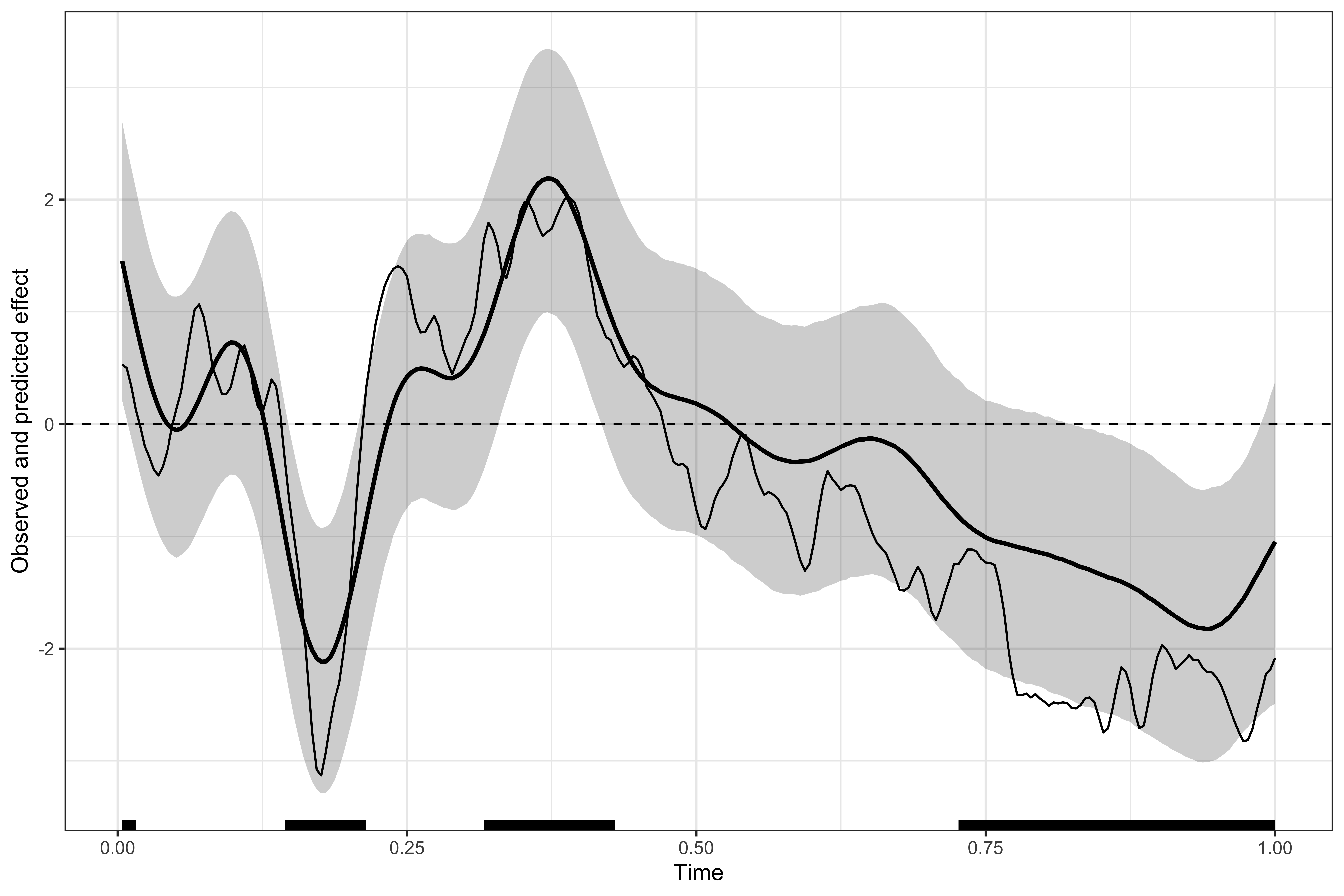
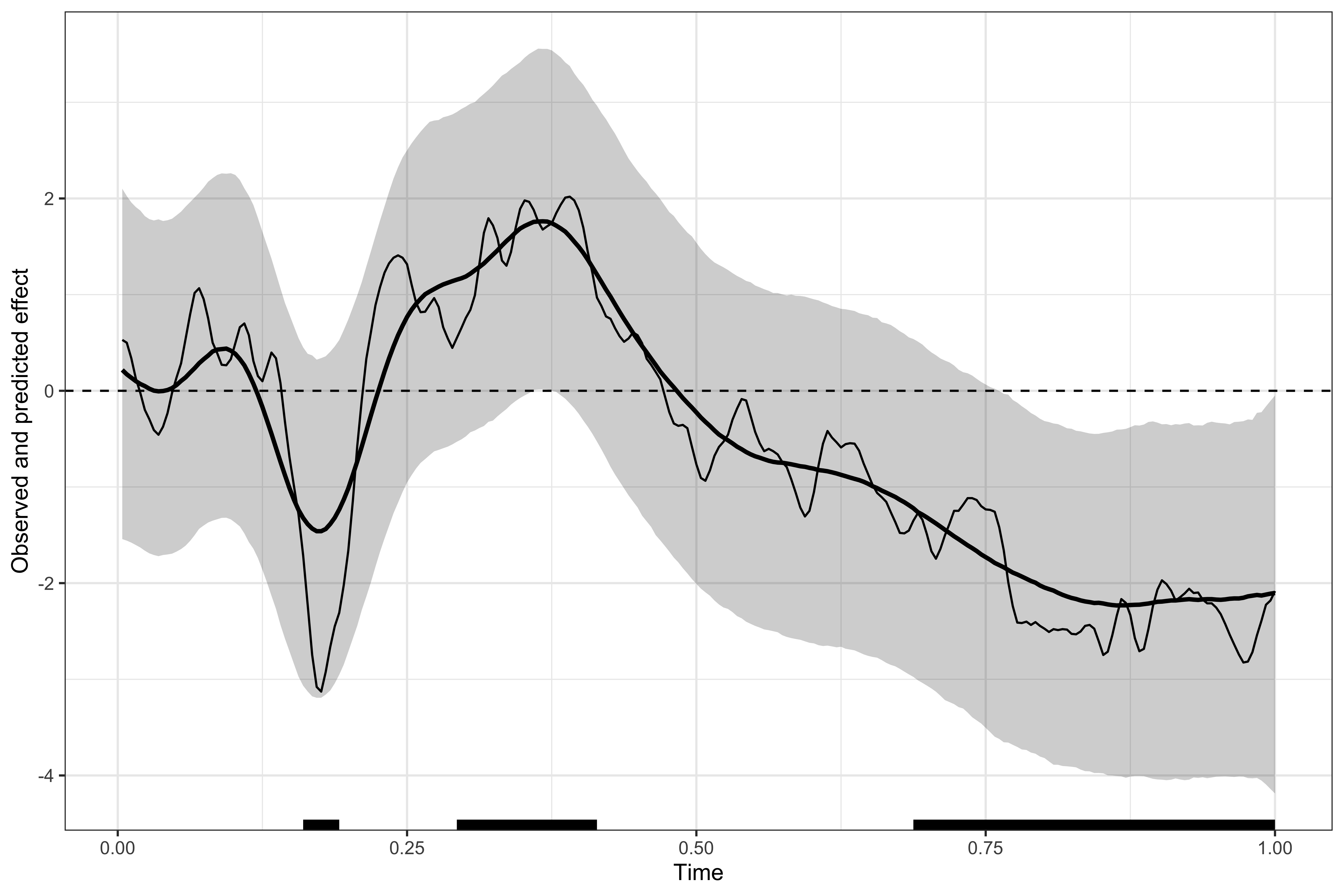
# plotting the data, model's predictions, and clusters
plot(results1)
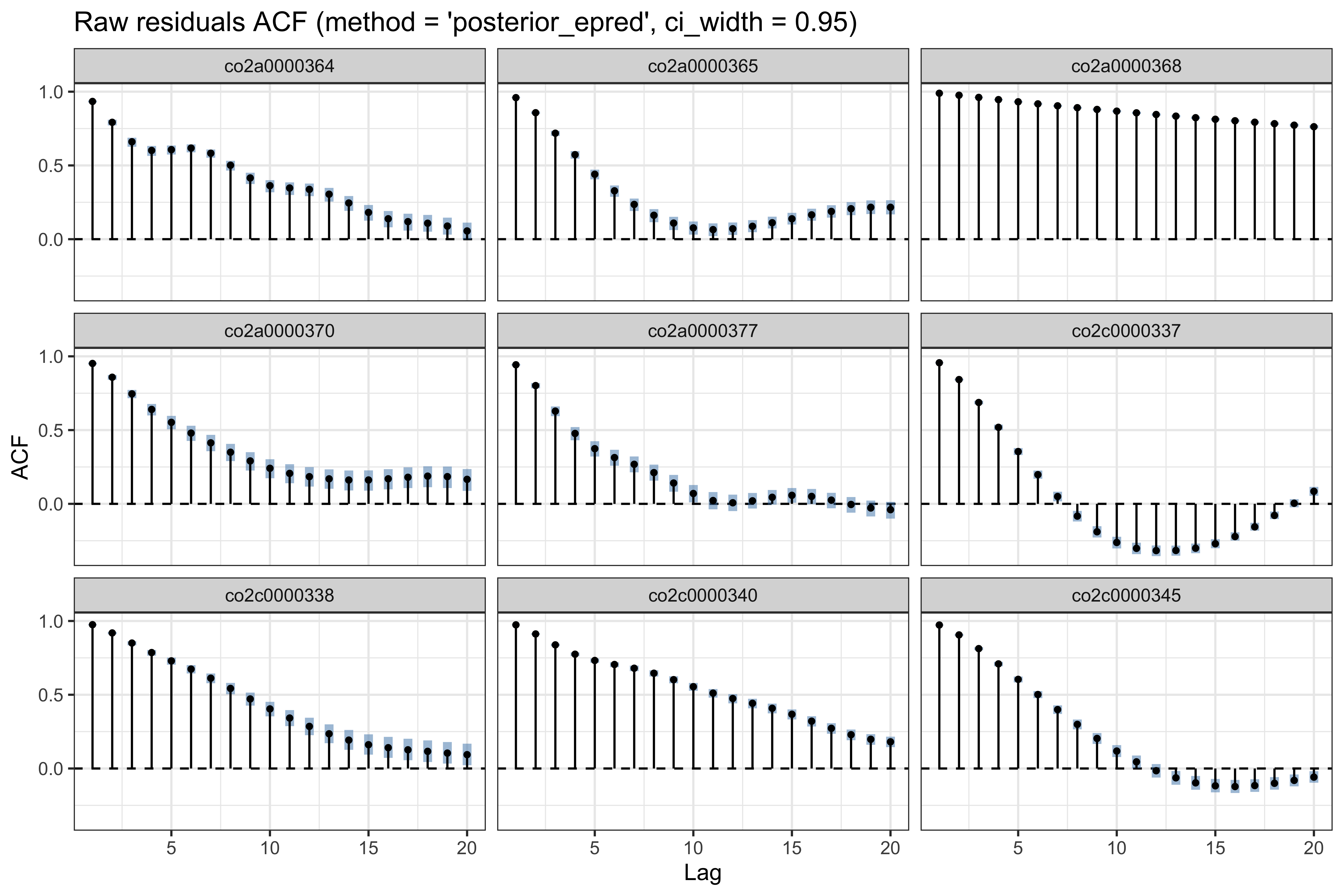
Checking auto-correlation
Below we use the check_residual_autocorrelation() function to check to residual auto-correlation. The ACF plot (per participant) reveals strong residual auto-correlation.
# checking residual auto-correlation
ar_check1 <- check_residual_autocorrelation(
    fit = results1$model
    )

# residual ACF (for some participants)
ar_check1$plots$acf_raw
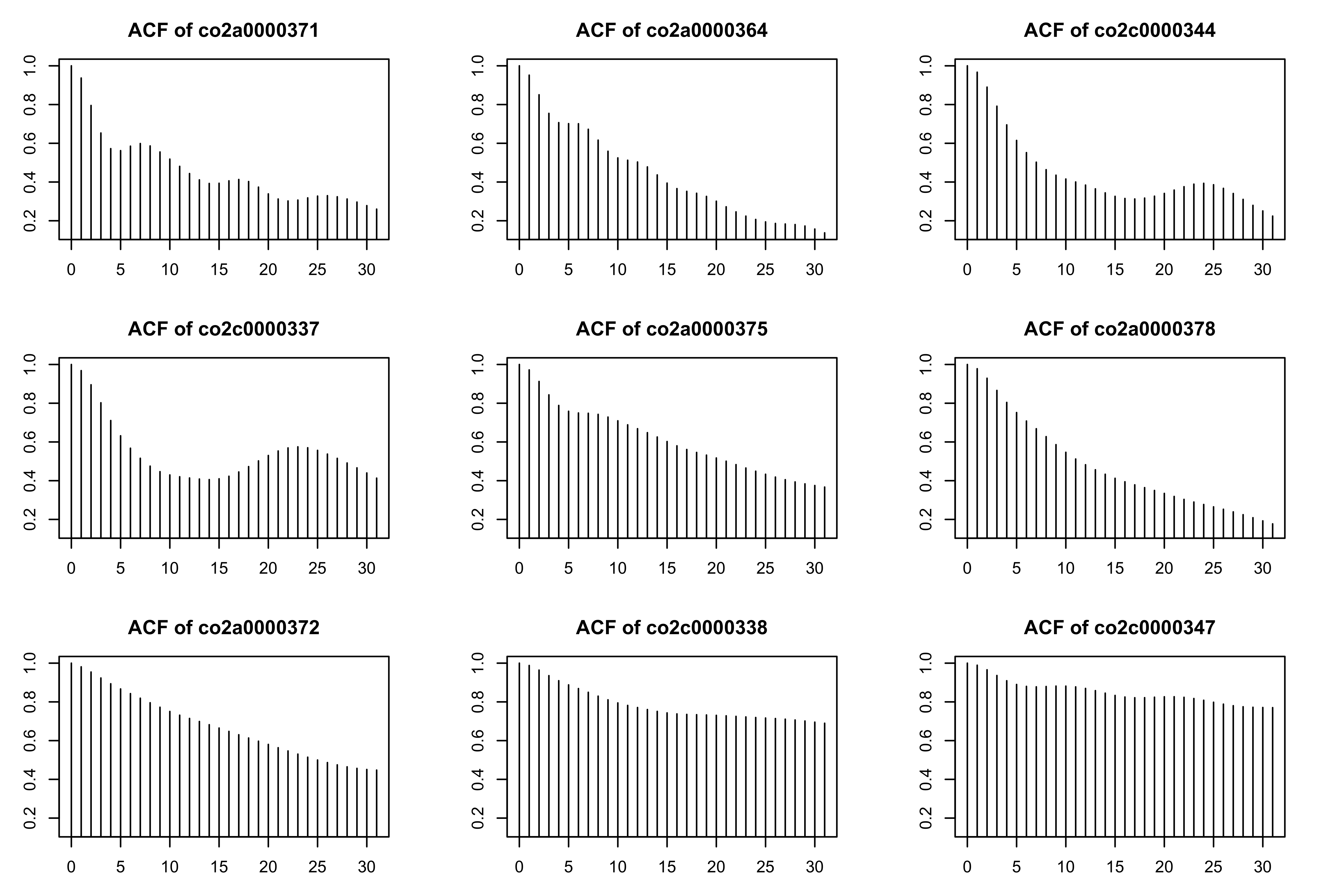
Compare with the residuals of the equivalent mgcv model (see also this vignette).
library(itsadug)
library(mgcv)

# fitting an equivalent mgcv model
m1 <- bam(voltage ~ s(time, k = 20) + s(subject, bs = "re"), data = eeg_data)

# plotting the raw residuals for some participants
acf_resid(model = m1, split_pred = "subject", n = 9)
#> Quantiles to be plotted:
#>        0%     12.5%       25%     37.5%       50%     62.5%       75%     87.5%
#> 0.9369281 0.9544371 0.9663653 0.9684141 0.9711032 0.9778108 0.9819698 0.9875842
#>      100%
#> 0.9893055
Modelling auto-correlation
The testing_through_time() function allows including a latent AR1 model to capture unmodelled autocorrelation (via include_ar_term = TRUE), which is estimated simultaneously to the other model parameters. This contrast with conventional approaches using a 2-step procedure consisting in first estimating the residual auto-correlation (from a first model), and then including this correlation as a fixed parameter in a subsequent model. Our approach, while more computationally intense, has several advantages:
Proper uncertainty propagation. Estimating the latent AR term jointly with the smooth/linear effects propagates uncertainty about autocorrelation into all model parameters and predictions. In contrast, a 2-step “estimate then fix it” approach is a plug-in procedure that conditions on an uncertain quantity, which may yield overconfident intervals (too-small SEs / under-coverage).
Less bias from mean-correlation confounding. Residual autocorrelation depends on what the mean model has already explained (and on smoothing penalties). When estimating autocorrelation from residuals of an initial fit, we risk misallocating structure between the smooth trend and the AR process. Joint estimation helps the model decide, probabilistically, whether variation is better explained by the smooth component or by autocorrelated deviations.
Cleaner, less error-prone prediction. Two-step workflows often require awkward post-hoc steps (fit trend, extract residuals, fit AR model, forecast residuals, back-transform, etc.), which is tedious and easy to get wrong. A joint latent AR formulation gives a single coherent generative model for estimation and prediction (see also this blogpost).
# fitting the BGAMM to identify clusters
results2 <- testing_through_time(
    # EEG data
    data = eeg_data,
    # participant column
    participant_id = "subject",
    # EEG column
    outcome_id = "voltage",
    # no predictor
    predictor_id = NA,
    # basis dimension
    kvalue = 20,
    # we recommend fitting the GAMM on summary statistics (mean and SD)
    multilevel = "summary",
    # no by-participant varying smooth (for speed purposes)
    varying_smooth = FALSE,
    # including (estimating) auto-correlation within the same model
    include_ar_term = TRUE,
    # threshold on posterior odds
    threshold = 10,
    # number of MCMCs
    chains = 4,
    # number of parallel cores
    cores = 4,
    # number of warmup iterations
    warmup = 1000,
    # total number of iterations (per chain)
    iter = 2000
    )
# checking residual auto-correlation
ar_check2 <- check_residual_autocorrelation(fit = results2$model)

# checking auto-correlation estimates
ar_check2$ar_summary
#>   parameter     mean          sd      q025      q50     q975
#> 1     ar[1] 0.992964 0.002707108 0.9862315 0.993497 0.996675
If the AR term correctly captured residual auto-correlation, we expect the average lag-1 auto-correlation to be lower in the corrected residuals than in the raw residuals.
head(x = ar_check2$rho1_by_series_raw)
#> # A tibble: 6 × 3
#>   .series     n_time  rho1
#>   <fct>        <int> <dbl>
#> 1 co2a0000364    256 0.944
#> 2 co2a0000365    256 0.961
#> 3 co2a0000368    256 0.997
#> 4 co2a0000369    256 0.962
#> 5 co2a0000370    256 0.969
#> 6 co2a0000371    256 0.970
head(x = ar_check2$rho1_by_series_corrected)
#> # A tibble: 6 × 3
#>   .series     n_time  rho1
#>   <fct>        <int> <dbl>
#> 1 co2a0000364    256 0.608
#> 2 co2a0000365    256 0.803
#> 3 co2a0000368    256 0.688
#> 4 co2a0000369    256 0.831
#> 5 co2a0000370    256 0.708
#> 6 co2a0000371    256 0.669

# average lag-1 autocorrelation across series
mean(x = ar_check2$rho1_by_series_raw$rho1, na.rm = TRUE)
#> [1] 0.9705104
mean(x = ar_check2$rho1_by_series_corrected$rho1, na.rm = TRUE)
#> [1] 0.7431609
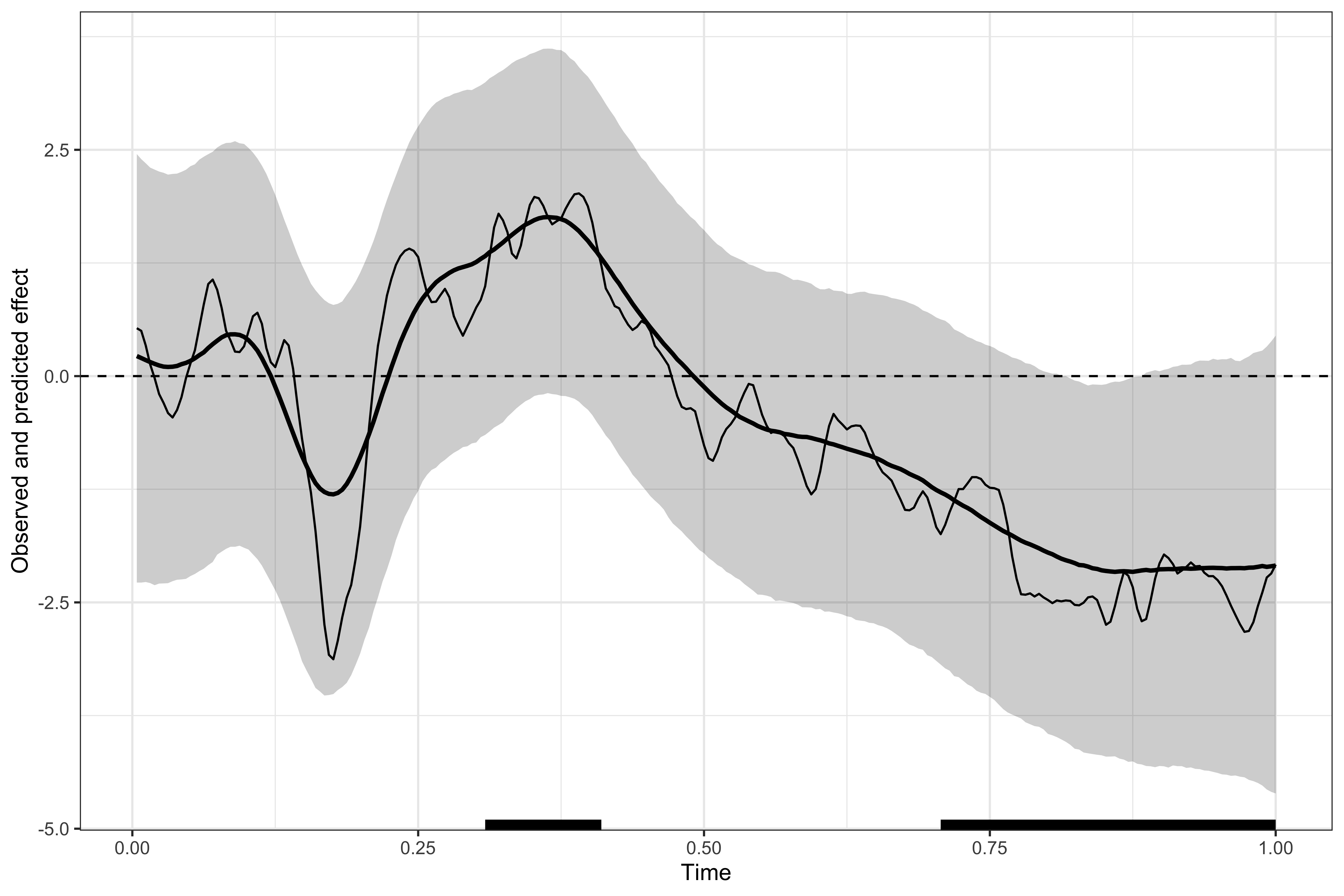
We then visualise the identified clusters, showing that this model produces much more conservative estimates (because of the larger uncertainty about group-level estimates.)
# displaying the identified clusters
print(results2)
#>
#> ==== Time-resolved GAM results ================================
#>
#> Clusters found: 3
#>
#>      sign id onset offset duration
#>  positive  1 0.293  0.414    0.121
#>  negative  1 0.160  0.191    0.031
#>  negative  2 0.688  1.000    0.312
#>
#> =================================================================
# plotting the data, model's predictions, and clusters
plot(results2)
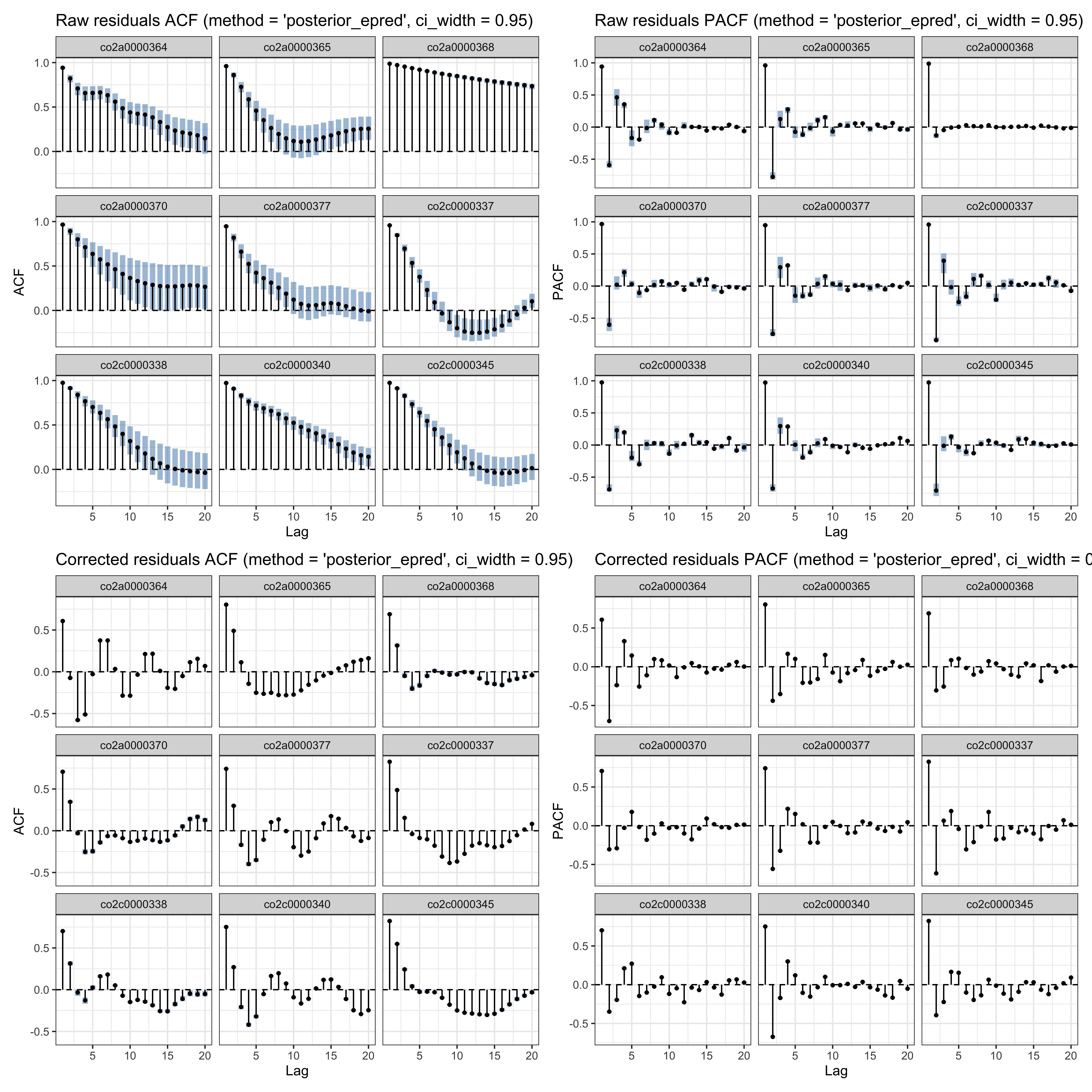
We visualise both the auto-correlation (ACF) and partial auto-correlation (pACF) of the raw and AR-corrected (whitened) residuals.
(ar_check2$plots$acf_raw + ar_check2$plots$pacf_raw) /
    (ar_check2$plots$acf_corrected + ar_check2$plots$pacf_corrected)
Model comparison
Model comparison suggests that the second model has much better out-of-sample predictive accuracy (lower WAIC).
# model comparison using WAIC
brms::waic(results1$model, results2$model)
#> Output of model 'results1$model':
#>
#> Computed from 4000 by 5120 log-likelihood matrix.
#>
#>           Estimate   SE
#> elpd_waic -13778.9 44.0
#> p_waic        39.8  4.1
#> waic       27557.8 88.0
#>
#> 12 (0.2%) p_waic estimates greater than 0.4. We recommend trying loo instead.
#>
#> Output of model 'results2$model':
#>
#> Computed from 4000 by 5120 log-likelihood matrix.
#>
#>           Estimate   SE
#> elpd_waic -12923.9 38.1
#> p_waic         1.1  0.1
#> waic       25847.9 76.1
#>
#> Model comparisons:
#>                elpd_diff se_diff
#> results2$model    0.0       0.0
#> results1$model -855.0      33.0
Lowering auto-correlation with varying smooth
Another way of reducing residual auto-correlation is to improve the model fit to capture finer structure present in the data. Below we show that auto-correlation can be considerably lowered by including per-participant varying smoothers.
# fitting the BGAMM to identify clusters
results3 <- testing_through_time(
    # EEG data
    data = eeg_data,
    # participant column
    participant_id = "subject",
    # EEG column
    outcome_id = "voltage",
    # no predictor
    predictor_id = NA,
    # basis dimension
    kvalue = 20,
    # we recommend fitting the GAMM on summary statistics (mean and SD)
    multilevel = "summary",
    # no by-participant varying smooth (for speed purposes)
    varying_smooth = TRUE,
    # threshold on posterior odds
    threshold = 10,
    # number of MCMCs
    chains = 4,
    # number of parallel cores
    cores = 4,
    # number of warmup iterations
    warmup = 1000,
    # total number of iterations (per chain)
    iter = 2000
    )
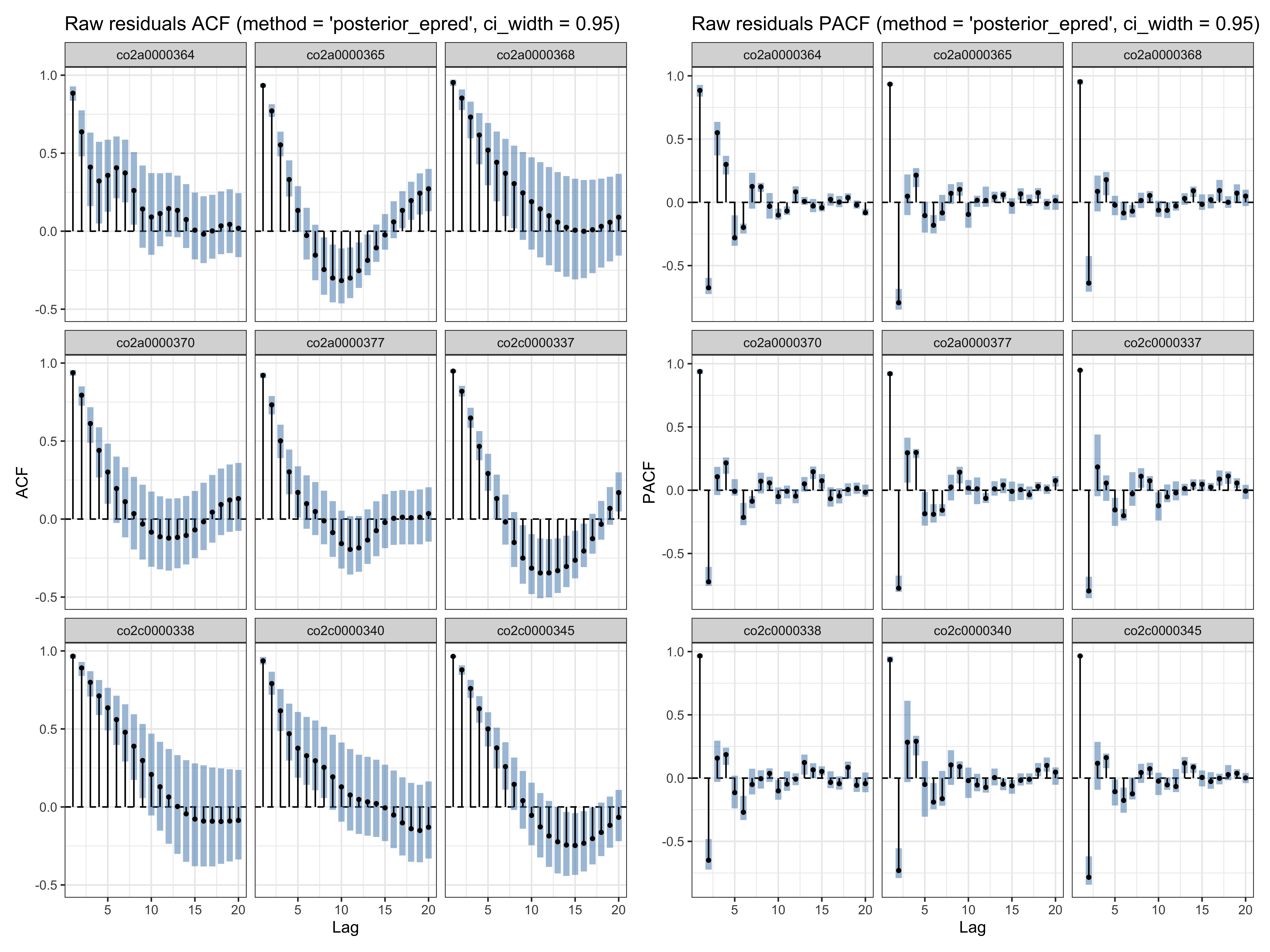
# checking residual auto-correlation
ar_check3 <- check_residual_autocorrelation(fit = results3$model)

# residual ACF and pACF (for some participants)
ar_check3$plots$acf_raw + ar_check3$plots$pacf_raw
# displaying the identified clusters
print(results3)
#>
#> ==== Time-resolved GAM results ================================
#>
#> Clusters found: 2
#>
#>      sign id onset offset duration
#>  positive  1 0.309   0.41    0.101
#>  negative  1 0.707   1.00    0.293
#>
#> =================================================================
# plotting the data, model's predictions, and clusters
plot(results3)
Model comparison
Model comparison suggests that this last model has slightly better out-of-sample predictive accuracy (lower WAIC).
# model comparison using WAIC
brms::waic(results1$model, results2$model, results3$model)
#> Output of model 'results1$model':
#>
#> Computed from 4000 by 5120 log-likelihood matrix.
#>
#>           Estimate   SE
#> elpd_waic -13778.3 44.0
#> p_waic        39.2  4.0
#> waic       27556.7 88.0
#>
#> 12 (0.2%) p_waic estimates greater than 0.4. We recommend trying loo instead.
#>
#> Output of model 'results2$model':
#>
#> Computed from 4000 by 5120 log-likelihood matrix.
#>
#>           Estimate   SE
#> elpd_waic -12923.9 38.1
#> p_waic         1.1  0.1
#> waic       25847.8 76.1
#>
#> Output of model 'results3$model':
#>
#> Computed from 4000 by 5120 log-likelihood matrix.
#>
#>           Estimate   SE
#> elpd_waic -12919.2 38.4
#> p_waic        37.6  1.9
#> waic       25838.5 76.7
#>
#> 4 (0.1%) p_waic estimates greater than 0.4. We recommend trying loo instead.
#>
#> Model comparisons:
#>                elpd_diff se_diff
#> results3$model    0.0       0.0
#> results2$model   -4.7       2.2
#> results1$model -859.1      33.1