Importing and visualising EEG data
Below we import and reshape EEG data from the eegkit package.
library(neurogam)
library(ggplot2)
library(eegkit)
library(dplyr)
# retrieving some EEG data
data(eegdata)
head(eegdata)
#> subject group condition trial channel time voltage
#> 1 co2a0000364 a S1 0 FP1 0 -8.921
#> 2 co2a0000364 a S1 0 FP1 1 -8.433
#> 3 co2a0000364 a S1 0 FP1 2 -2.574
#> 4 co2a0000364 a S1 0 FP1 3 5.239
#> 5 co2a0000364 a S1 0 FP1 4 11.587
#> 6 co2a0000364 a S1 0 FP1 5 14.028
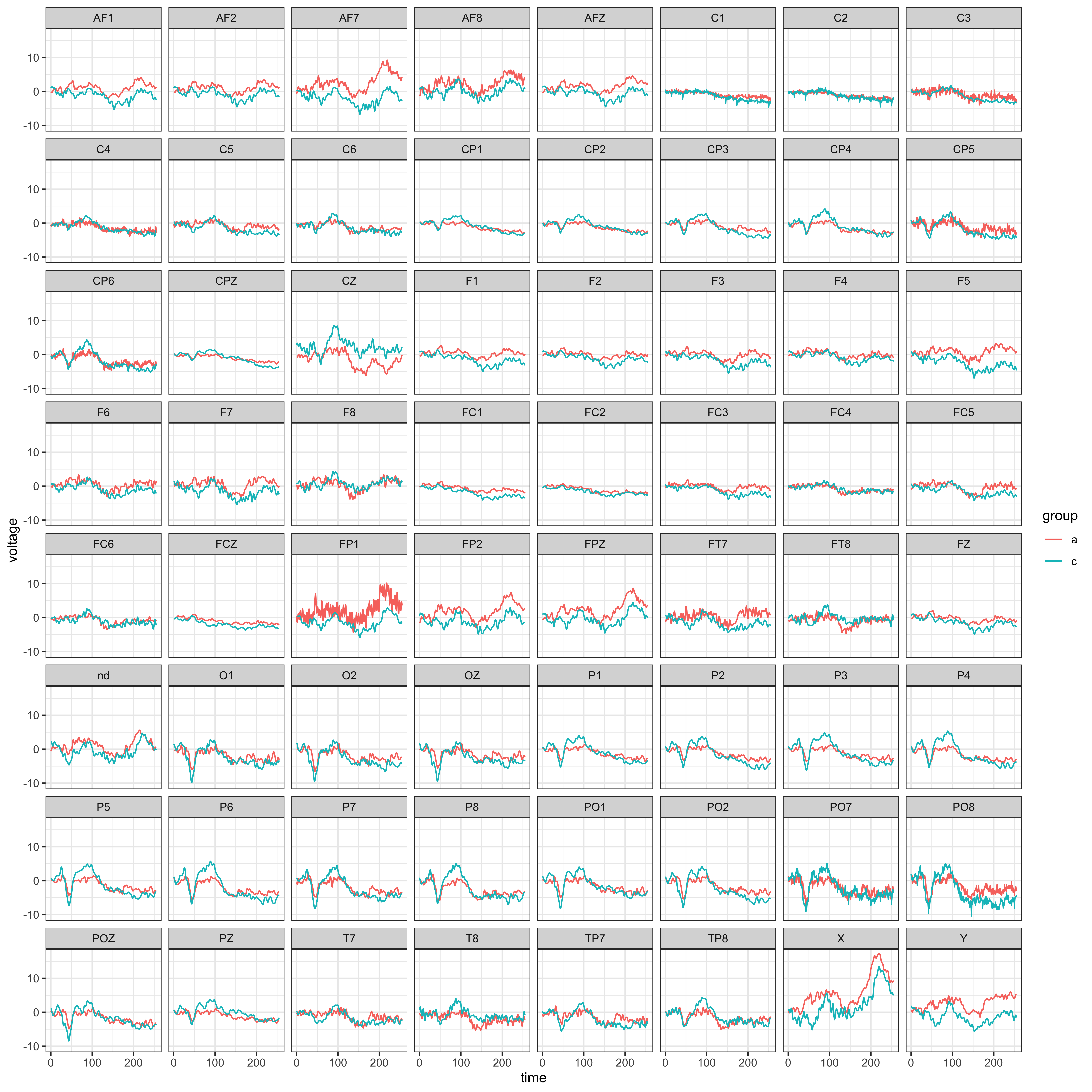
# plotting the average ERP per group and channel
eegdata |>
summarise(voltage = mean(voltage), .by = c(group, channel, time) ) |>
ggplot(aes(x = time, y = voltage, colour = group) ) +
geom_line() +
facet_wrap(~channel) +
theme_bw()
# reshape the data
eeg_data <- eegdata |>
    # keeping only one channel
    dplyr::filter(channel == "PZ") |>
    # converting timesteps to seconds
    mutate(time = (time + 1) / 256) |>
    # rounding numeric variables
    mutate(across(where(is.numeric), ~ round(.x, 4) ) ) |>
    # removing NAs
    na.omit()

# show a few rows
head(eeg_data)
#>       subject group condition trial channel   time voltage
#> 1 co2a0000364     a        S1     0      PZ 0.0039  -2.797
#> 2 co2a0000364     a        S1     0      PZ 0.0078  -4.262
#> 3 co2a0000364     a        S1     0      PZ 0.0117  -4.262
#> 4 co2a0000364     a        S1     0      PZ 0.0156  -2.797
#> 5 co2a0000364     a        S1     0      PZ 0.0195  -0.844
#> 6 co2a0000364     a        S1     0      PZ 0.0234   0.132
Fitting the model
We fit the model (a BGAMM) on one channel (PZ) to test for group difference at every timestep.
# fitting the BGAMM to identify clusters (around 30 min on 4 parallel apple M4 cores)
results <- testing_through_time(
    # EEG data
    data = eeg_data,
    # participant column
    participant_id = "subject",
    # EEG column
    outcome_id = "voltage",
    # name of predictor in data
    predictor_id = "group",
    # basis dimension
    kvalue = 40,
    # we recommend fitting the GAMM on summary statistics (mean and SD)
    multilevel = "summary",
    # threshold on posterior odds
    threshold = 10,
    # number of MCMCs
    chains = 4,
    # number of parallel cores
    cores = 4
    )
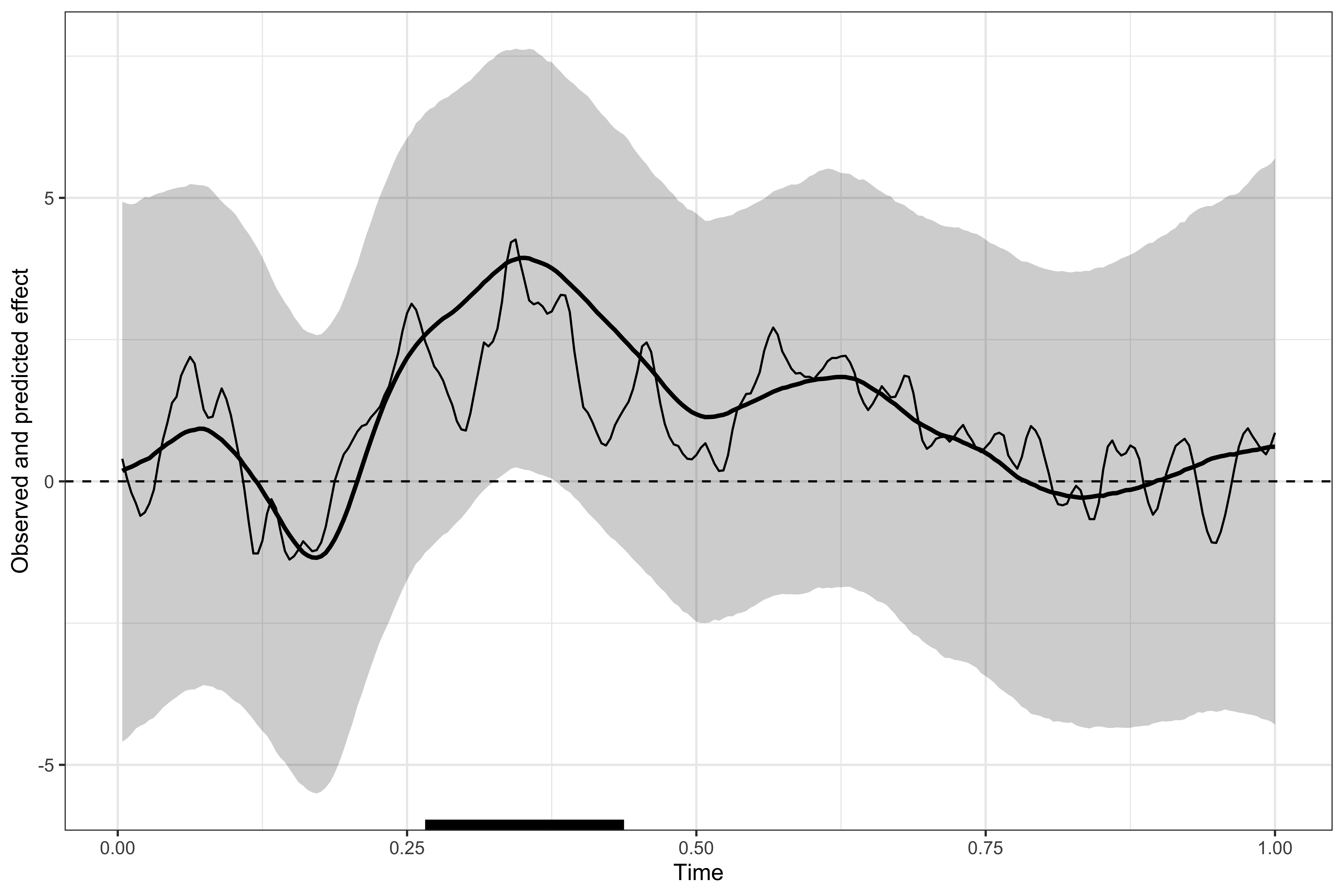
Visualising the results
# displaying the identified clusters
print(results)
#>
#> ==== Time-resolved GAMM results ===============================
#>
#> Clusters found:
#>
#>      sign id onset offset duration
#>  positive  1 0.266  0.438    0.172
#>
#> =================================================================
# plotting the data, model's predictions, and clusters
plot(results)
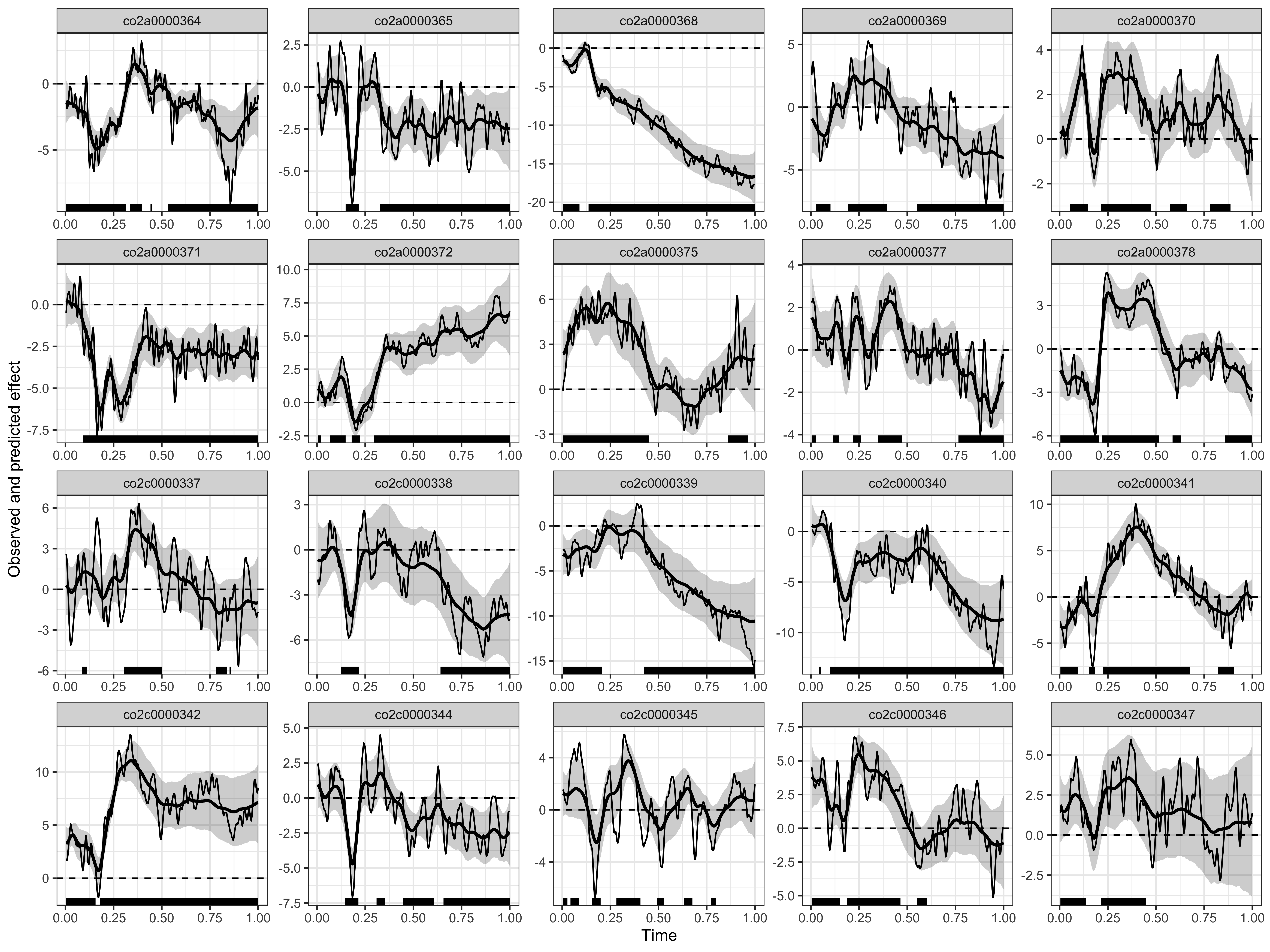
Computing clusters at the participant-level
Below we fit a new model, specifying predictor_id = NA (because group varies across participants) and by_ppt = TRUE to test whether EEG amplitude (voltage) differs from 0 and return clusters at the participant level.
# fitting the BGAMM to identify clusters (around 30 min on 4 parallel apple M4 cores)
results <- testing_through_time(
    # EEG data
    data = eeg_data,
    # participant column
    participant_id = "subject",
    # EEG column
    outcome_id = "voltage",
    # here we use no predictor (because group varies across participants)
    predictor_id = NA,
    # basis dimension (for both the group and participant levels)
    kvalue = 40,
    # we recommend fitting the GAMM with summary statistics (mean and SD)
    multilevel = "summary",
    # return clusters at both the group and participant levels
    by_ppt = TRUE,
    # threshold on posterior odds
    threshold = 10,
    # number of MCMCs
    chains = 4,
    # number of parallel cores
    cores = 4
    )
Visualising the results
# displaying the identified clusters
print(results)
#>
#> ==== Time-resolved GAMM results ===============================
#>
#> Clusters found:
#>
#>  participant     sign id onset offset duration
#>  co2a0000364 positive  1 0.336  0.398    0.062
#>  co2a0000364 negative  1 0.004  0.312    0.308
#>  co2a0000364 negative  2 0.441  0.449    0.008
#>  co2a0000364 negative  3 0.531  1.000    0.469
#>  co2a0000365 negative  1 0.148  0.219    0.071
#>  co2a0000365 negative  2 0.328  1.000    0.672
#>  co2a0000368 negative  1 0.004  0.090    0.086
#>  co2a0000368 negative  2 0.137  1.000    0.863
#>  co2a0000369 positive  1 0.191  0.394    0.203
#>  co2a0000369 negative  1 0.027  0.102    0.075
#>  co2a0000369 negative  2 0.551  1.000    0.449
#>  co2a0000370 positive  1 0.055  0.148    0.093
#>  co2a0000370 positive  2 0.215  0.473    0.258
#>  co2a0000370 positive  3 0.574  0.660    0.086
#>  co2a0000370 positive  4 0.781  0.887    0.106
#>  co2a0000371 negative  1 0.090  1.000    0.910
#>  co2a0000372 positive  1 0.004  0.020    0.016
#>  co2a0000372 positive  2 0.066  0.148    0.082
#>  co2a0000372 positive  3 0.297  1.000    0.703
#>  co2a0000372 negative  1 0.180  0.223    0.043
#>  co2a0000375 positive  1 0.004  0.449    0.445
#>  co2a0000375 positive  2 0.859  0.965    0.106
#>  co2a0000377 positive  1 0.004  0.027    0.023
#>  co2a0000377 positive  2 0.113  0.144    0.031
#>  co2a0000377 positive  3 0.219  0.258    0.039
#>  co2a0000377 positive  4 0.348  0.473    0.125
#>  co2a0000377 negative  1 0.766  1.000    0.234
#>  co2a0000378 positive  1 0.219  0.516    0.297
#>  co2a0000378 negative  1 0.004  0.203    0.199
#>  co2a0000378 negative  2 0.586  0.629    0.043
#>  co2a0000378 negative  3 0.789  0.789    0.000
#>  co2a0000378 negative  4 0.859  1.000    0.141
#>  co2c0000337 positive  1 0.086  0.113    0.027
#>  co2c0000337 positive  2 0.305  0.500    0.195
#>  co2c0000337 negative  1 0.781  0.840    0.059
#>  co2c0000337 negative  2 0.852  0.859    0.007
#>  co2c0000338 negative  1 0.125  0.219    0.094
#>  co2c0000338 negative  2 0.641  1.000    0.359
#>  co2c0000339 negative  1 0.004  0.207    0.203
#>  co2c0000339 negative  2 0.426  1.000    0.574
#>  co2c0000340 positive  1 0.043  0.051    0.008
#>  co2c0000340 negative  1 0.098  1.000    0.902
#>  co2c0000341 positive  1 0.227  0.676    0.449
#>  co2c0000341 negative  1 0.004  0.094    0.090
#>  co2c0000341 negative  2 0.152  0.184    0.032
#>  co2c0000341 negative  3 0.820  0.906    0.086
#>  co2c0000342 positive  1 0.004  0.156    0.152
#>  co2c0000342 positive  2 0.180  1.000    0.820
#>  co2c0000344 positive  1 0.246  0.246    0.000
#>  co2c0000344 positive  2 0.309  0.352    0.043
#>  co2c0000344 negative  1 0.144  0.215    0.071
#>  co2c0000344 negative  2 0.445  0.606    0.161
#>  co2c0000344 negative  3 0.656  1.000    0.344
#>  co2c0000345 positive  1 0.004  0.027    0.023
#>  co2c0000345 positive  2 0.043  0.086    0.043
#>  co2c0000345 positive  3 0.281  0.406    0.125
#>  co2c0000345 positive  4 0.633  0.676    0.043
#>  co2c0000345 negative  1 0.156  0.199    0.043
#>  co2c0000345 negative  2 0.492  0.527    0.035
#>  co2c0000345 negative  3 0.773  0.797    0.024
#>  co2c0000346 positive  1 0.004  0.152    0.148
#>  co2c0000346 positive  2 0.188  0.465    0.277
#>  co2c0000346 negative  1 0.551  0.602    0.051
#>  co2c0000347 positive  1 0.004  0.137    0.133
#>  co2c0000347 positive  2 0.215  0.449    0.234
#>
#> =================================================================
# plotting the data, model's predictions, and clusters
plot(results)
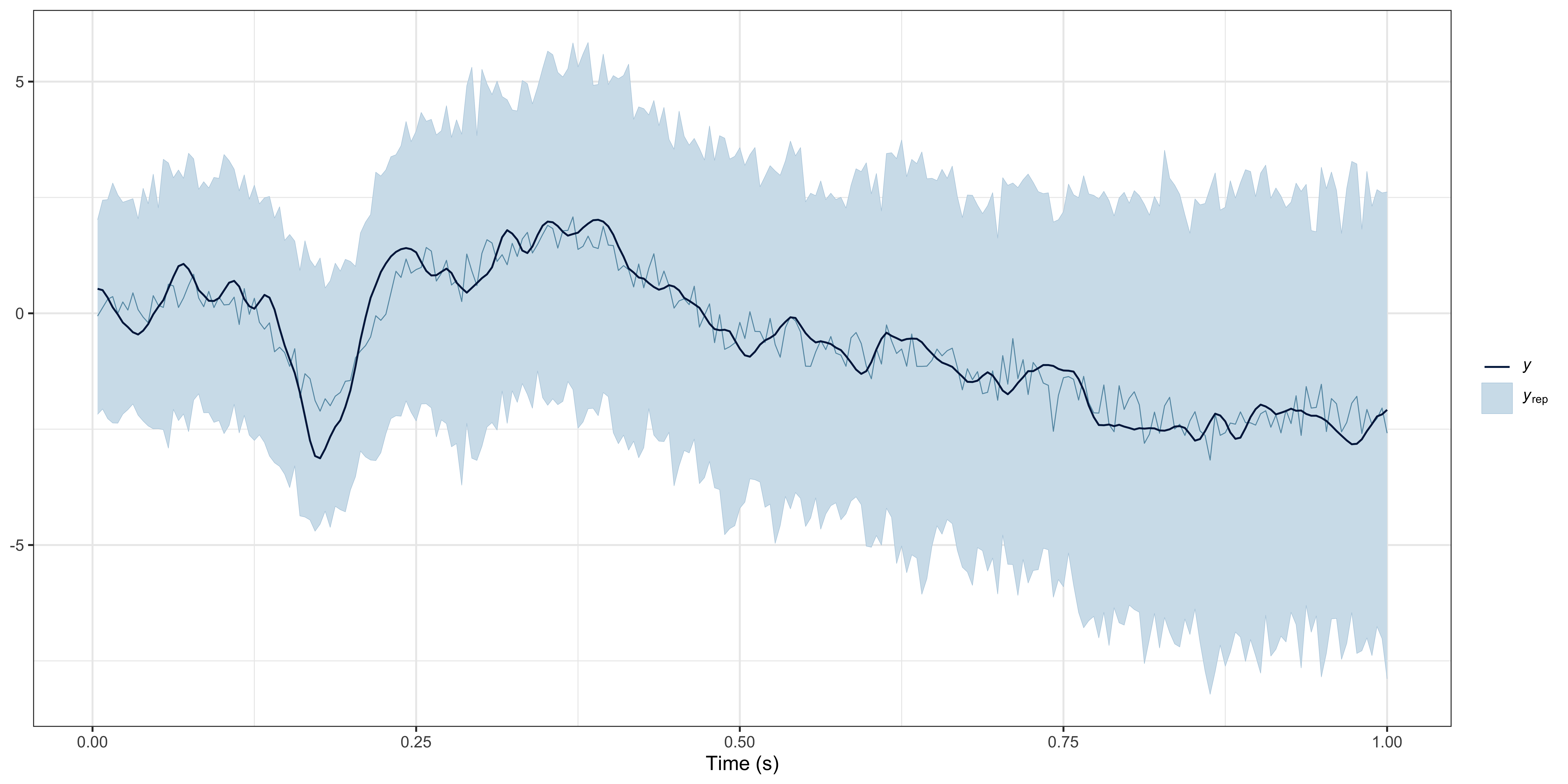
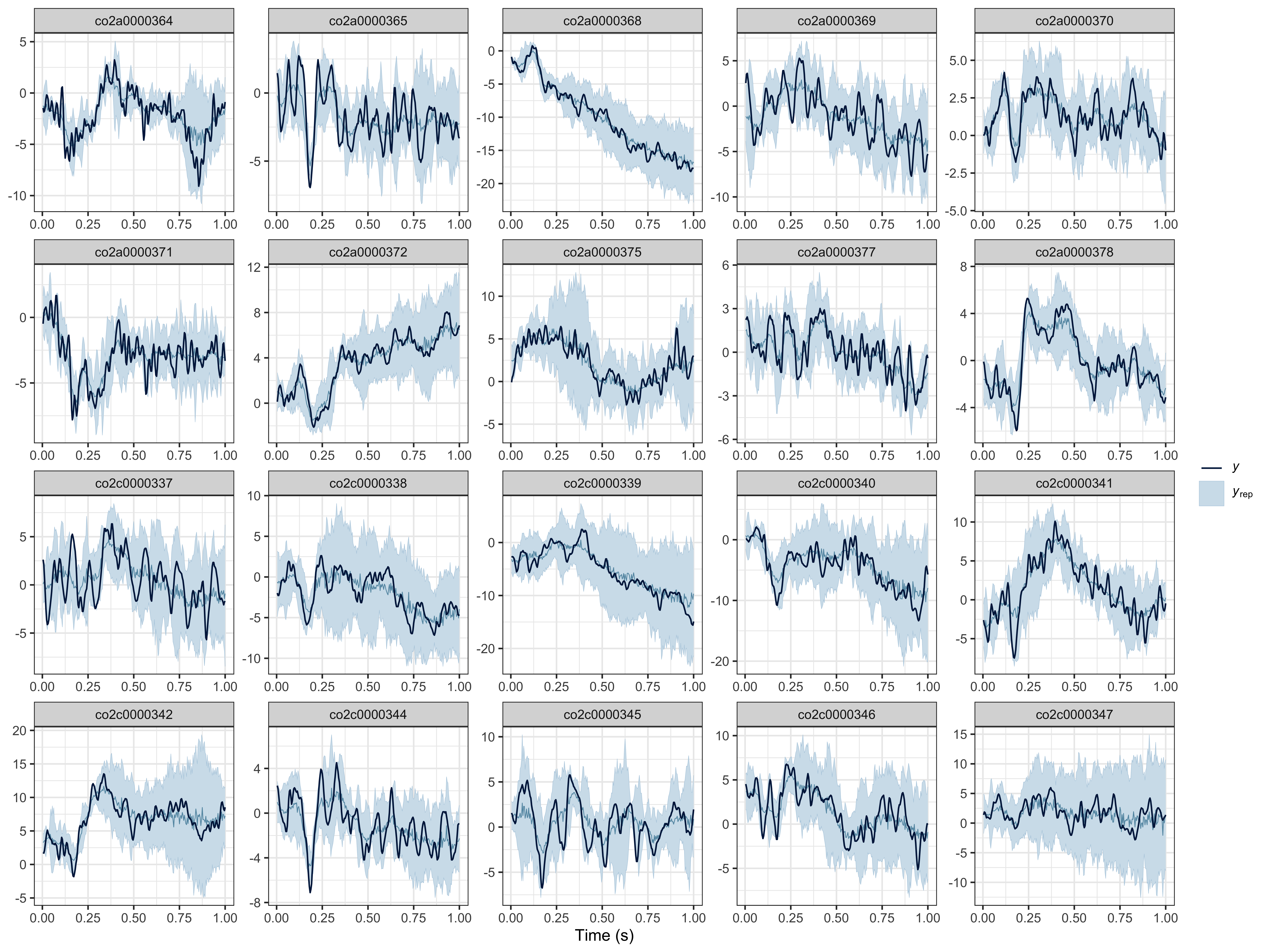
Posterior predictive checks
We recommend visually assessing the predictions of the model against the observed data (for each participant). We provide a lightweight ppc() method, but you can conduct various PPCs with brms::pp_check(results$model, ...) (for all available PPCs, see https://mc-stan.org/bayesplot/reference/PPC-overview.html).
# posterior predictive checks (PPCs) at the group level
ppc(object = results, ppc_type = "group")
# posterior predictive checks (PPCs) at the participant level
ppc(object = results, ppc_type = "participant")