Importing and visualising the data
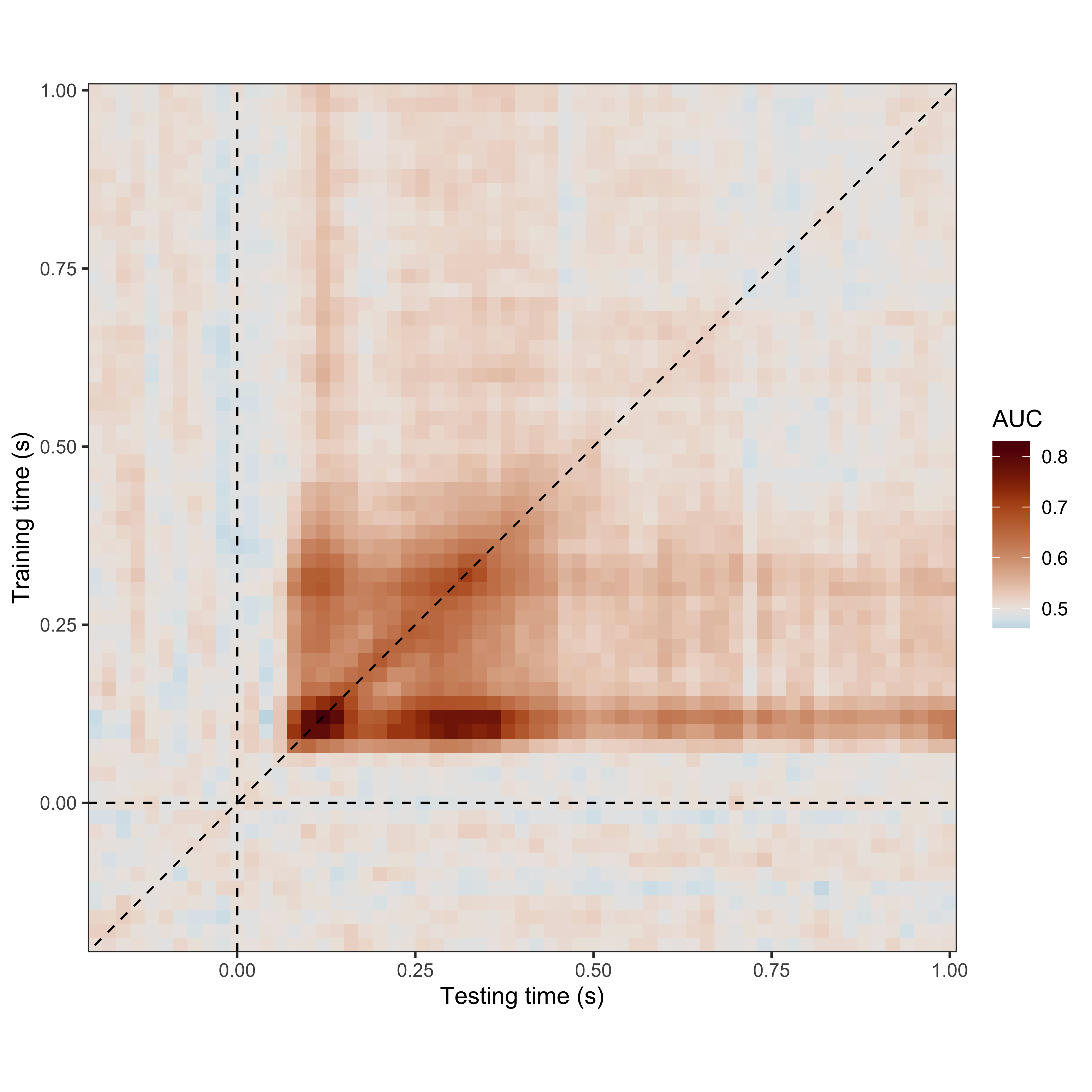
Below we import and visualise the cross-temporal decoding generalisation data discussed in Nalborczyk & Bürkner (2025, Appendix A).
library(neurogam)
library(ggplot2)
library(scico)
library(dplyr)

# retrieving some EEG data
data(timegen_data)
head(timegen_data)
#>   train_time test_time       auc participant
#> 1       -0.2      -0.2 0.5639503           1
#> 2       -0.2      -0.2 0.5967508           2
#> 3       -0.2      -0.2 0.4648438           3
#> 4       -0.2      -0.2 0.4935377           4
#> 5       -0.2      -0.2 0.5228509           5
#> 6       -0.2      -0.2 0.4771995           6

# plotting the cross-temporal generalisation matrix
timegen_data |>
    summarise(auc = mean(auc), .by = c(train_time, test_time) ) |>
    ggplot(aes(x = train_time, y = test_time, fill = auc) ) +
    geom_tile() +
    geom_vline(xintercept = 0, linetype = 2, linewidth = 0.5) +
    geom_hline(yintercept = 0, linetype = 2, linewidth = 0.5) +
    geom_abline(slope = 1, intercept = 0, linetype = 2, linewidth = 0.5) +
    scale_x_continuous(expand = c(0, 0) ) +
    scale_y_continuous(expand = c(0, 0) ) +
    coord_fixed() +
    theme_bw() +
    scico::scale_fill_scico(palette = "vik", midpoint = 0.5, name = "AUC") +
    labs(x = "Testing time (s)", y = "Training time (s)")
Fitting the model
We fit a 2D BGAMM (with a varying intercept, but no varying smooth) to identify clusters with above-chance decoding accuracy. Such models are much slower than 1D temporal models, we recommend running less chains and using within-chain parallelisation (as shown below with threads = threading(threads = 4)) We also recommend to start with simple models (e.g., low kvalue, no varying effect) to be able to diagnose potential issues rapidly. For more details on such models, see for instance Pedersen et al. (2019).
library(brms)

# fitting a BGAMM with two temporal dimensions
timegen_gam <- brm(
    formula = auc ~ t2(train_time, test_time, bs = "tp", k = 25) + (1 | participant),
    data = timegen_data,
    warmup = 1000,
    iter = 3000,
    chains = 2,
    cores = 2,
    backend = "cmdstanr",
    threads = threading(threads = 4),
    stan_model_args = list(stanc_options = list("O1") )
    )
Identifying clusters
The previous model is equivalent to the following testing_through_time() call. This model takes around 15 hours on 8 parallel apple M4 cores.
# we compute the smallest effect size of interest (SESOI) as the baseline
# (i.e., before stimulus onset) upper 95% quantile of AUC values
baseline_upper_quantile <- timegen_data %>%
    filter(train_time < 0 & test_time < 0) %>%
    summarise(quantile(x = auc, probs = 0.95) ) %>%
    pull()

# fitting the BGAMM to identify clusters
results <- testing_through_time(
    # cross-temporal generalisation data
    data = timegen_data,
    # participant column
    participant_id = "participant",
    # AUC column
    outcome_id = "auc",
    # testing against chance level
    predictor_id = NA,
    # defining training and testing times
    time_id = c("train_time", "test_time"),
    # basis dimension
    kvalue = 25,
    # only includes a per-participant varying intercept (no varying smooth)
    multilevel = "summary",
    use_se = FALSE,
    varying_smooth = FALSE,
    # defining chance level for AUC values
    # chance_level = 0.5,
    # defining chance level + SESOI (upper AUC values during baseline)
    chance_level = baseline_upper_quantile,
    # threshold on posterior odds
    threshold = 10,
    # testing whether AUC is above chance
    threshold_type = "above",
    # number of warmup iterations
    warmup = 1000,
    # total number of iterations (per chain)
    iter = 3000,
    # number of MCMCs
    chains = 2,
    # number of parallel cores
    cores = 2,
    # using with-chain parallelisation (needs 2x4 parallel cores)
    threads = brms::threading(threads = 4),
    # increasing max_treedepth
    stan_control = list(max_treedepth = 15)
    )
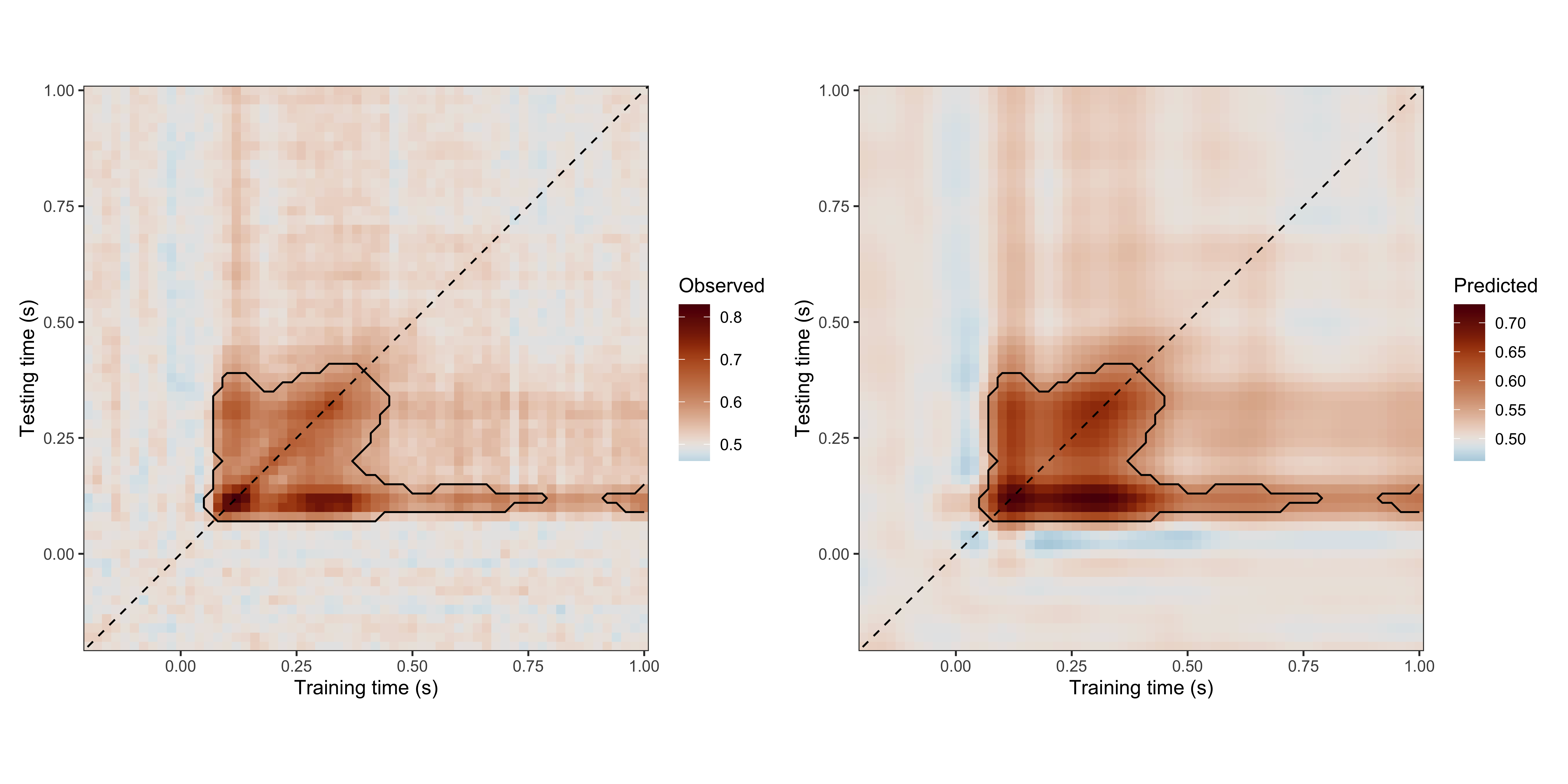
The results can be summarised and visualised using the dedicated print(), summary(), and plot() methods.
# print a summary table ("value" represents the posterior odds)
print(results)
#>
#> ==== Time-resolved GAM results ================================
#>
#> Clusters found: 2
#>
#>      sign id onset_time1 onset_time2 offset_time1 offset_time2 span_time1
#>  positive  1        0.06        0.08         0.78         0.40       0.72
#>  positive  2        0.92        0.10         1.00         0.14       0.08
#>  span_time2 n_points value_min value_max
#>        0.32      317     10.08  4000.000
#>        0.04        9     13.44   332.333
#>
#> =================================================================

# for available colour palettes, see scico::scico_palette_show()
plot(
    x = results,
    palette = "vik", midpoint = 0.5,
    axes_labels = c("Training time (s)", "Testing time (s)")
    )